SPLAT Plotting Routines
These are the primary plotting routines for SPLAT, which allow visualization of spectral data and comparison to other templates and models. Additional routines to visualize indices on the spectral data and index values themselves are currently under development
plotSpectrum
SPLAT allows spectrophotometry of spectra using common filters in the red optical and near-infrared. The filter transmission files are stored in the SPLAT reference library, and are accessed by name. A list of current filters can be made by through the ``plotSpectrum()``_ routine:
The core plotting function is ``plotSpectrum()``_, which allows flexible methods for displaying single or groups of spectra, and comparing spectra to each other. This codes are built around the routines in matplotlib, and the API has the full list of options.
Simple plots
Simple
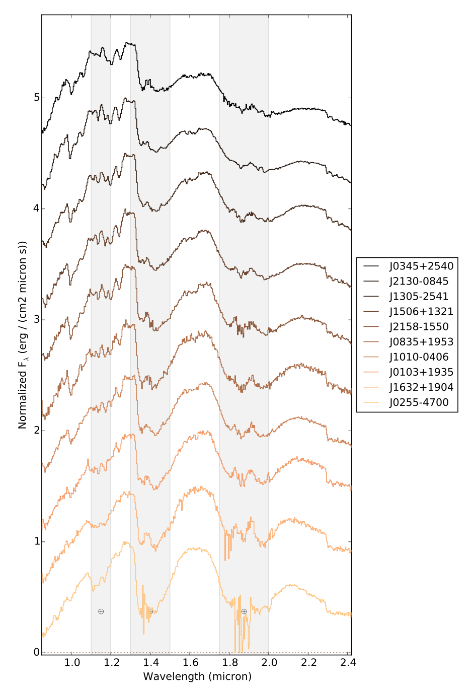
Plotting multiple spectra
Spectra can be stacked on top of each other using the stack parameter, which is a numerical value that indicates the offset between
Comparison plots
Legends, feature labels and other additions
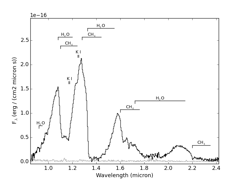
- Specific absorption features can be labeled on the plot setting the
featuresto a list of atoms and molecules. The features currently contained in the code include: - r’H$_2$O’: bands at 0.92-0.95, 1.08-1.20, 1.33-1.55, and 1.72-2.14 micron
- r’CH$_4$’: bands at 1.10-1.24, 1.28-1.44, 1.60-1.76, and 2.20-2.35 micron
- r’CO’: band at 2.29-2.39
- r’TiO’: bands at 0.76-0.80 and 0.825-0.831 micron
- r’VO’: band at 1.04-1.08 micron
- r’FeH’: bands at 0.98-1.03, 1.19-1.25, and 1.57-1.64 micron
- r’H$_2$’: broad absorption over 1.5-2.4 micron
- r’H I’: lines at 1.004, 1.093, 1.281, 1.944, and 2.166 micron
- r’Na I’: lines at 0.819, 1.136, and 2.21 micron
‘nai’: {‘label’: r’Na I’, ‘type’: ‘line’, ‘wavelengths’: [[0.8186,0.8195],[1.136,1.137],[2.206,2.209]]}, ‘na1’: {‘label’: r’Na I’, ‘type’: ‘line’, ‘wavelengths’: [[0.8186,0.8195],[1.136,1.137],[2.206,2.209]]}, ‘mg’: {‘label’: r’Mg I’, ‘type’: ‘line’, ‘wavelengths’: [[1.7113336,1.7113336],[1.5745017,1.5770150],[1.4881595,1.4881847,1.5029098,1.5044356],[1.1831422,1.2086969],]}, ‘mgi’: {‘label’: r’Mg I’, ‘type’: ‘line’, ‘wavelengths’: [[1.7113336,1.7113336],[1.5745017,1.5770150],[1.4881595,1.4881847,1.5029098,1.5044356],[1.1831422,1.2086969],]}, ‘mg1’: {‘label’: r’Mg I’, ‘type’: ‘line’, ‘wavelengths’: [[1.7113336,1.7113336],[1.5745017,1.5770150],[1.4881595,1.4881847,1.5029098,1.5044356],[1.1831422,1.2086969],]}, ‘ca’: {‘label’: r’Ca I’, ‘type’: ‘line’, ‘wavelengths’: [[2.263110,2.265741],[1.978219,1.985852,1.986764],[1.931447,1.945830,1.951105]]}, ‘cai’: {‘label’: r’Ca I’, ‘type’: ‘line’, ‘wavelengths’: [[2.263110,2.265741],[1.978219,1.985852,1.986764],[1.931447,1.945830,1.951105]]}, ‘ca1’: {‘label’: r’Ca I’, ‘type’: ‘line’, ‘wavelengths’: [[2.263110,2.265741],[1.978219,1.985852,1.986764],[1.931447,1.945830,1.951105]]}, ‘caii’: {‘label’: r’Ca II’, ‘type’: ‘line’, ‘wavelengths’: [[1.184224,1.195301],[0.985746,0.993409]]}, ‘ca2’: {‘label’: r’Ca II’, ‘type’: ‘line’, ‘wavelengths’: [[1.184224,1.195301],[0.985746,0.993409]]}, ‘al’: {‘label’: r’Al I’, ‘type’: ‘line’, ‘wavelengths’: [[1.672351,1.675511],[1.3127006,1.3154345]]}, ‘ali’: {‘label’: r’Al I’, ‘type’: ‘line’, ‘wavelengths’: [[1.672351,1.675511],[1.3127006,1.3154345]]}, ‘al1’: {‘label’: r’Al I’, ‘type’: ‘line’, ‘wavelengths’: [[1.672351,1.675511],[1.3127006,1.3154345]]}, ‘fe’: {‘label’: r’Fe I’, ‘type’: ‘line’, ‘wavelengths’: [[1.5081407,1.5494570],[1.25604314,1.28832892],[1.14254467,1.15967616,1.16107501,1.16414462,1.16931726,1.18860965,1.18873357,1.19763233]]}, ‘fei’: {‘label’: r’Fe I’, ‘type’: ‘line’, ‘wavelengths’: [[1.5081407,1.5494570],[1.25604314,1.28832892],[1.14254467,1.15967616,1.16107501,1.16414462,1.16931726,1.18860965,1.18873357,1.19763233]]}, ‘fe1’: {‘label’: r’Fe I’, ‘type’: ‘line’, ‘wavelengths’: [[1.5081407,1.5494570],[1.25604314,1.28832892],[1.14254467,1.15967616,1.16107501,1.16414462,1.16931726,1.18860965,1.18873357,1.19763233]]}, ‘k’: {‘label’: r’K I’, ‘type’: ‘line’, ‘wavelengths’: [[0.7699,0.7665],[1.169,1.177],[1.244,1.252]]}, ‘ki’: {‘label’: r’K I’, ‘type’: ‘line’, ‘wavelengths’: [[0.7699,0.7665],[1.169,1.177],[1.244,1.252]]}, ‘k1’: {‘label’: r’K I’, ‘type’: ‘line’, ‘wavelengths’: [[0.7699,0.7665],[1.169,1.177],[1.244,1.252]]}} ‘sb’: {‘label’: r’*’, ‘type’: ‘band’, ‘wavelengths’: [[1.6,1.64]]},
telluric- labels the regions of strong telluric absorption
Legends are handled in the same manner
Examples
- Example 1: A simple view of a random spectrum
This example shows various ways of displaying a random spectrum in the library
>>> import splat
>>> spc = splat.getSpectrum(spt = 'T5', lucky=True)[0]   # select random spectrum
>>> spc.plot()                                                   # this automatically generates a "quicklook" plot
>>> splat.plotSpectrum(spc)                                      # does the same thing
>>> splat.plotSpectrum(spc,uncertainty=True,tdwarf=True)     # show the spectrum uncertainty and T dwarf absorption features
The last plot should look like the following:
- Example 2: Compare two spectra
Optimally scale and compare two spectra.
>>> import splat
>>> spc = splat.getSpectrum(spt = 'T5', lucky=True)[0]   # select random spectrum
>>> spc2 = splat.getSpectrum(spt = 'T4', lucky=True)[0]  # read in another random spectrum
>>> comp = splat.compareSpectra(spc,spc2)        # compare spectra to get optimal scaling
>>> spc2.scale(comp[1])                  # apply optimal scaling
>>> splat.plotSpectrum(spc,spc2,colors=['black','red'],labels=[spc.name,spc2.name])     # show the spectrum uncertainty and T dwarf absorption features
- Example 3: Compare several spectra for a given object
In this case we’ll look at all of the spectra of TWA 30B in the library, sorted by year and compare each to the first epoch data. This is an example of using both multiplot and multipage.
>>> splist = splat.getSpectrum(name = 'TWA 30B')         # get all spectra of TWA 30B
>>> junk = [sp.normalize() for sp in splist]             # normalize the spectra
>>> dates = [sp.date for sp in splist]                   # observation dates
>>> spsort = [s for (d,s) in sorted(zip(dates,splist))]   # sort spectra by dates
>>> dates.sort()                                         # don't forget to sort dates!
>>> splat.plotSpectrum(spsort,multiplot=True,layout=[2,2],multipage=True,\   # here's our plot statement
    comparison=spsort[0],uncertainty=True,mdwarf=True,telluric=True,legends=dates,\
    legendLocation='lower left',output='TWA30B.pdf')
Here is the first page of the resulting 5 page pdf file

- Example 4: Display the spectra sequence of L dwarfs